You can use the Excel Index and Match formulas to match and find data in an Excel spreadsheet. Included is a free Excel download that shows exactly how to use Index Match
This is the first in a series of posts explaining Excel features quickly and simply. If you find it easier to understand concepts with a working example, opt-in below and download a fully working Index Match formula example that shows step-by-step how to compare two columns in Excel.
The INDEX and MATCH functions, when used together work like a better version of a VLOOKUP. Read on for a quick summary of what the template above shows explains with working examples.
General Problem
How to find and return the value from one column, based on the value in different column.
Problem Detail
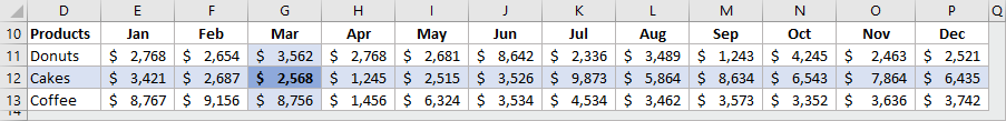
In the table below, I want to get the sales figure for Cakes in March.
Use Index Match to find the value for Cakes in March
Quick Solution
=INDEX(G11:G13, MATCH("Cakes", D11:D13, 0))
Explanation
The MATCH formula returns the relative position of a value within a range of values. In the example above, MATCH("Cakes", D11:D13, 0) will return the number 2, meaning the second row in the range D11 to D13.
The INDEX formula returns a single value from a range of values, based on the relative row number. In the example above INDEX(G11:G13, MATCH("Cakes", D11:D13, 0)) returns the second row in the range G11 to G13 because the MATCH function returns the number 2.
Did you know ... that automating your documents and spreadsheet can save you hundreds of hours of wasted time? MergeOS makes it easy to automatically generate reports and other documents using Word and Excel files. Try it out for free for 2 week here.